Abstract

This project involved deriving valuable information around genetical variations by analysing a large dataset on powerlighting. Data mining models were created primarily using Python and the machine learning and data mining toolkit 'Orange'.

Powerlifting Dataset

The chosen dataset for this study is the ‘OpenPowerLifting’ dataset, found through Kaggle, a platform for predictive modelling, containing thousands of validated datasets.

This dataset contains large amounts of data, in a comma separated value (CSV) format, which were extracted from meets (competitions) and competitor results in the sport of powerlifting, where competitors compete to lift the most weight for their class in three separate weightlifting categories: bench pressing, squats and deadlifts. Demographic data on meets, such as location and dates are also included, alongside the large quantity of competitor result data (386,415 total).

Data Pre-processing

Before analysis on the dataset occurred, certain pre-processing and data cleaning was required.

The data from the CSV files were inputting into an SQLite3 database, rows with 'blank' data values were deleted and Python scripts were created to merge both data files together with the corrosponding primary keys.

Normalisation on names, locations and other string formatted datapoints was also done to eliminate differences within user-input.

Classification using Neural Networks

For this project, a neural network was developed using Python to classify competitors as male or female based on all the powerlifting variables (Weight lifted, Age, Height, Weight, Wilks, etc...

Modules are imported in lines 1, 2 and 3. Here, we are using the Keras package, used for developing and evaluating deep learning models. Keras wraps numerical computation libraries, such as Theano and TensorFlow, allowing for the development of machine learning models.

NumPy is also used to add support for large, multi-dimensional arrays and matrices. NumPy also provides a large collection of high-level mathematical functions to operate arrays.

Training and testing data are imported and assigned to variables. For training, the target variable is assigned to its own variable (line 7). Note: For this model, the dataset was changed slightly, and now uses integers and floats only (0 or 1 instead of males and females).

from keras.models import Sequential
from keras.layers import Dense
import numpy as np

trainset = numpy.loadtxt("nntraindata.csv", delimiter=",")
X = trainset[:,0:7]
Y = trainset[:,7]

Next, we define the neural network model. The input layer is assigned to 7 inputs. Here we use a fully-connected network structure with three layers (2 hidden layers).

The number of neurons within each layer are defined in the first argument and set the activation functions.

The ‘sigmoid’ function is used on the output layer to ensure the network output is Boolean, of either 0 or 1.

model = Sequential()
model.add(Dense(64, input_dim=7, init='uniform', activation='relu'))
model.add(Dense(128, init='uniform', activation='relu'))
model.add(Dense(64, init='uniform', activation='sigmoid'))

The model is then compiled:

• The loss function ‘binary_crossentropy’, a logarithmic loss, is used to evaluate a set of weights. This is a good default loss function, and we are hoping for loss to go down after every epoch.


• The optimiser ‘adam’, an efficient gradient descent algorithm, is used to search through different weights for the network. Again, 'adam' is a good default optimiser to use. Later, once I'm more familer of the inner workings of optimisers, I will be able to implement and test different ones.


• The metrics are used to print out accuracy reports during training, demonstrating the model improving.



Epochs are a fixed number of training iterations through the dataset, and the batch size argument sets the number of instances that are evaluated before a weight is updated in the network. Lowering the batch size is recommended for large datasets, where RAM capacity is a limitation.

‘Model.predict()’ is used for testing and making predictions. With the sigmoid activation function in the output layer, predictions will range from 0 to 1 (male or female).

model.compile(loss='binary_crossentropy', optimizer='adam', metrics=['accuracy'])
model.fit(X, Y, epochs=10, batch_size=64)
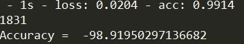
predictions = model.predict(test_data)

Once finished, the model was able to predict genders at an accuracy of 98.9%. This slight difference may be the result of changing the optimisation functions, using three network layers, batch size, or other network metrics.

The ability to customise and develop machine learning algorithms from scratch using Python has many advantages over Orange, and in large scale projects is definitely the superior method.



---

Which country is powerlifting most popular in?

The data consists of a total of 8482 meets, held from 1974 – 2018.

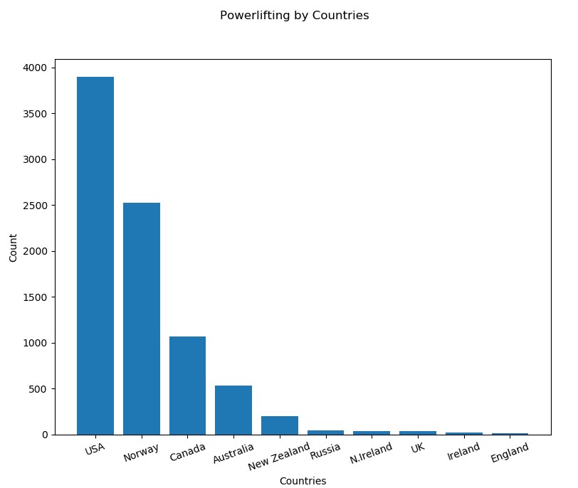
Python was used here to iterate through the meets dataset and calculate the top 10 countries, by adding a count to a country in a dictionary for each iteration.

def process_data(data):
    country_dict = {}
    country_list = []

    for country in data:
        if country in country_dict:
            country_dict[country] += 1
        else:
            country_dict[country] = 1

    for a, b in country_dict.items():
        country_list.append([a[0], b])

    country_list = sorted(country_list,key=itemgetter(1), reverse=True)

    return country_list

Python was also used to visualise the data in a bar graph, using a module called ‘Matplotlib’, a plotting library for Python. The Python script displayed the graph and printed out the meet count for the top ten countries.

def bar_graph():
    names = []
    values = []
    count = 0

    for country, value in country_list:
            if count > 9:
                pass
            else:
                count = count + 1
                names.append(country)
                values.append(value)
            
    for value, name in zip(values, names):
        print(name, "meet count:", value)
        
    plt.figure(1, figsize=(9, 3))
    plt.subplot()
    plt.bar(names, values)
    plt.ylabel('Count')
    plt.xlabel('Countries')
    plt.xticks(rotation=20)
    plt.suptitle('Powerlifting by Countries')
    plt.show()
    
process_data(read_from_db())  
bar_graph()

The data produced clearly shows that USA, with 3894 meets, is the most popular country in terms of powerlifting, followed by 2521 in Norway. The UK only had a total of 34 meets, suggesting powerlifting is unpopular and not a traditional British sport. With a huge popularity in USA, it may indicate that USA has the most potential for winning Olympic events associated with powerlifting, as they will have the largest talent pool.



---

k-Means Clustering - Identifying Powerlifting genetic differences

Next, the k-Means algorithm was used on the data set to see where and what difference is there within different categories of powerlifting.

The k-Means algorithm is used here to automatically assign sub-classes to data and see how well it can split the data up into clusters, essentially separating the data into different classes.

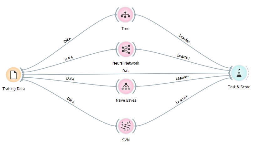
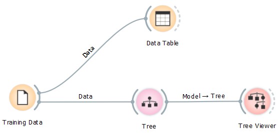
Orange was used here, using its unsupervised k-Means model. The reason for using Orange here was it can generate simple, yet effective visualisations of the output, plotting the data into a scatter plot graph.



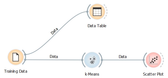
• Training Data – The imported CSV file.
• Data Table – Presents the dataset in a spreadsheet.
• k-Means – Clustering algorithm used to generate clusters.
• Scatter Plot – Visualisation widget used to visualise the output of the k-Means algorithm

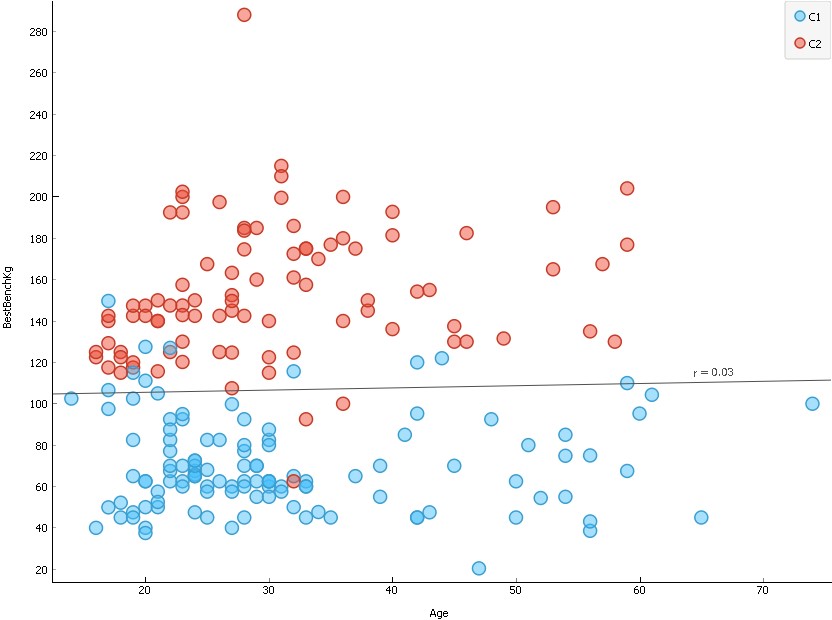
The first analysis was done on age and best bench score (see scatter plot below). The scatter plot shots two clusters, both with a clear separation, indicating the algorithm clearly identified two main differences in the dataset just from data on age and bench score.

The first cluster ranges from around 40 to 95, and the second cluster from 110 to 215. The average scores for male and female competitors in this dataset was 147kg and 66kg in the bench press respectively, suggesting that the first and second cluster belonged to female and male powerlifters respectively. Furthermore, the regression line generated was clearly in the middle of the two clusters, in the 105-110kg range.

These results show that there is a clear difference between Male and Females powerlifters regarding bench pressing, with Male lifters on average being able to score over double the weight.

Orange scatterplot visualisation output for age and bench press.



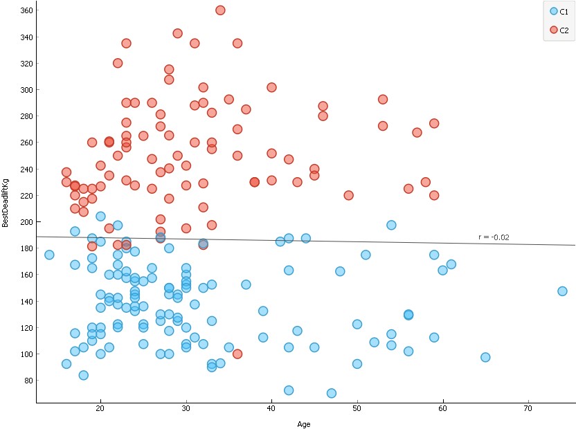
This method analysis was also done for deadlifting and similar results were produced (see scatter plot below).

For deadlifting, two clear clusters were generated. The average score for deadlifting for males and females were 237.5kg and 136.1kg respectively. The average data point in cluster 1 and 2 is around 130 and 270 respectively, suggesting that cluster 1 are female lifters and cluster 2 are male.

The implementation of the k-Means algorithm demonstrates its strength for automated clustering and was able to partition this dataset into two meaningful sub-classes.

Orange scatterplot visualisation output for age and deadlift.



---

Male or Female classification based lifting scores, age and bodyweight

Using data of age, bodyweight, all 3 lifting scores, total lifting score and wilks score as features, classification algorithms are applied and evaluated based on their ability to classify the input as male or females.

Which classification algorithm is best?

There were four main classification algorithms used for this study:

Decision Tree – A tree algorithm with forward pruning, which splits data into nodes by class purity.
Neural Network – A multi-layer perceptron (MLP) algorithm using backpropagation. In Orange, the neural network widget uses sklearns MLP algorithm.
Naïve Bayes – A simple probabilistic classifier based upon Bayes’ theorem. Naïve Bayes learns a Naïve Bayesian model from the data.
SVM s– Separates the attribute space with a hyperplane, often yields supreme predictive performance results.

All four of these algorithms were used in Orange. The full dataset was used here, and applied to each algorithm, where the sex data was set to the target, and other data fields were features.



The ‘Test and Score’ widget was used to calculate the performance of each classifier. This widget has the option to use a percentage of the data as training, and the rest for testing. It is important to separate training and testing data as testing machine learning algorithms with the same training data will produce biased results, as the algorithm will simply be able to produce results based on what it learnt during training. Here, 66% of the dataset was used for training.

The Test and Score widget displayed the following results for each algorithm:



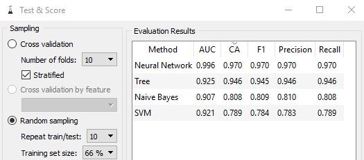
There are multiple different evaluation metrics produced. Here, we are mainly concerned with the classification accuracy (CA) metric, showing the percentage of correctly classified examples.

Neural networks scored a CA of 0.97 (97% accuracy), whereas SVM scored the lowest with only 0.784 (78.4%), clearly showing the power of neural networks and why it is considered the state-of-the-art. Surprising however, the decision tree also outperformed the SVM by a large margin. In this example, the full dataset was used, which is where the neural network shines, bringing up the question of how well will the neural network perform will a small amount of data?

Neural Network and SVM performance with less data

In the previous test we saw the power of the neural network with a large dataset. One of the predominate reasons on why neural networks have become so powerful is due to the increase and availability of data. By using its layers of computational units (neurons), with connections to neurons in other layers, neural networks can transform data using a series of computations until they can classify it as an output. An activation function is used with a threshold, used to adjust the neurons value when all connections are processed. This whole process requires large quantities of data to improve its algorithm over time.

The next test is the same as the previous, however it uses a small amount of data. Instead of the full dataset, a small portion of 200 instances will be used. The results are as follows:



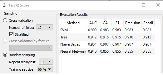
The above results show that, with the small amount of data, SVM significantly outperformed all other classification algorithms with a CA of 0.983, surprisingly increasing its CA over the previous test, with less data. The neural network scored a CA of 0.855, a decrease of 0.11% compared to the previous test.

---

Which powerlifting variable is the most influential in predicting gender?

It has already been made clear that there is a clear difference between male and females in powerlifting, but not so clear which variable is the most influential.

Orange includes a ‘Tree Viewer’ widget, a tool used to visualise the classification decisions of regression trees. Essentially, the Tree Viewer evaluates the decision tree classifier, and visualises the tree showing its logic.

This widget can be used to show which variables influence the decision tree the highest.

The Orange model used for this test is below:



At the top of the decision tree is the bench press variable:



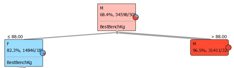
The tree shows that if the bench press variable is over 88, 96.5% of the time the competitor will be male, and if less than 88, 82.3% of the time Female. Being at the top of the decision tree, bench pressing is the most influential variable which determines whether a powerlifter is male or female, suggesting that out of the three powerlifting exercises, males are best at bench pressing. This also may suggest that males biologically have more upper body strength and grow stronger/ have the most potential for growth on pushing muscles (triceps, shoulders and chest) when compared to females.

If weight for the bench press is below 88, the decision tree then compares two other variables, age and Wilks:



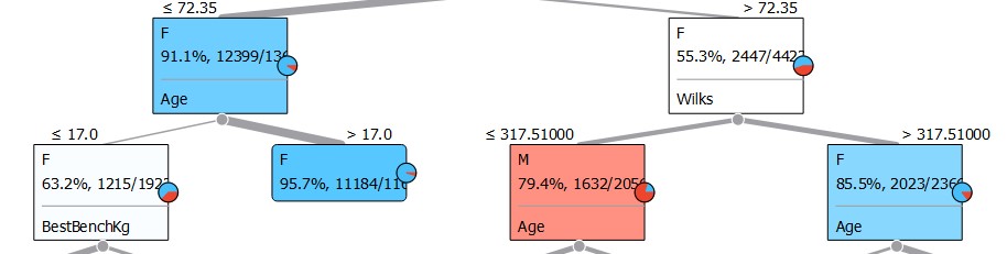
This layer of the decision tree shows if bench press is lower than 72.35, and age is greater than 17, then 95.7% of the time the competitor is female, otherwise it will again compare bench press again. On the other hand, if bench press is greater than 72.35, and Wilks score is lower than 317.5, 79.4% of the time the competitor will be female.

These results show that after bench pressing, age is the next influential variable which has the highest impact on powerlifting, suggesting that age has a strong effect on the performance of powerlifters.

The decision tree continues to expand to over 50 nodes, using different variables and values to classify competitors as male or female. In the screenshots taken, only the first few layers were shown.

---

Conclusion

In this project, many machine learning methods were applied to a messy dataset, resulting in stimulating and thought-provoking information being extracted. Multiple different instances of evidence were produced, showing the differences between males and females in powerlifting, and the difference between powerlifting exercises, age and bodyweight and the impact these variables have on powerlifting performance. Furthermore, the power of different machine learning models was demonstrated, specifically the dominance of artificial neural networks.

Further work can potentially be directed towards adding more data to the dataset used in this study, potentially comparing other physical and powerlifting factors such as height, powerlifting experience, disabilities, diet, etc. Information extracted from powerlifting data can be used to speed up scientific research in weight lifting and potentially be used # to develop powerlifting training programs to optimise growth for the next generation of powerlifters.  

---